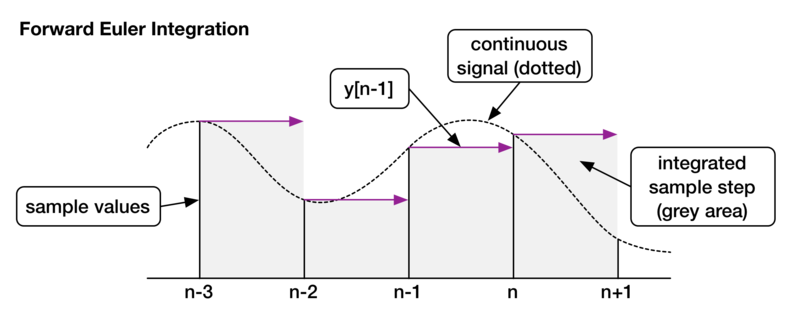
So I finally fired up OmniGraffle to sketch some examples for Forward Euler vs. Trapezoidal Integration. Let's dive right in:

The idea is, to integrate a known function y = f(x) we simply sample that function and build square blocks between the sample intervals. Those blocks are supposed to approximate the integral of that function. This is what we all know from lowpass filters which go like this:
s[n] = y[n-1]
y[n] = g * ( x[n] - y[n-1] ) + s[n]
At each sample instance we calculate a new value based on the input sample and a state that we assume to be equivalent to the previous sample value - which we stretch out to a rectangular block over the whole period of time that passed since the previous sample.
Note that we don't need to multiply y[n-1] with any time constant "t" whatsoever because the time constant is already "baked"into our coefficient g when we set it to something like 1 - exp(2 * PI * cutoff/samplerate). When we divide our frequency by the sample rate, we essentially "normalize" the time constant so that it becomes 1 for each instance. The grey area under the sample is then equivalent to 1 * y, and - if it wasn't too obvious - any muliplication by factor 1 is surplus.
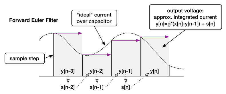
The difference to the above graphic of a function being integrated is, in a filter the result output of the next step depends on the integrated area of the current step. The function we're integrating in a RC filter is the current over the capacitor. That integral (i.e. the grey area) is the output voltage of a filter for each sample step.
Here's an adapted graph that shows how our filter output (grey area) corresponds to the current updates (function values) which are taken for the calculation of the next step:

Now, what we also see: That integrated area is really pretty far off from that below the perfectly continuous signal. We can hardly expect to get really close results for future samples when we base our computation on those staircase equivalent blocks. This is where the trapezoidal rule comes in.

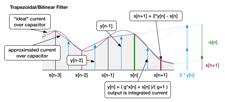
Check this out! - Instead of using a staircase analogy, we draw a straight line from one sample point to the other. Marvelously, the grey area matches the area below the perfectly continuous signal much better than the previous method.
But how do we get there? - As I wrote in my previous blog entry, at first glance we need to look into the future. But actually we don't. By solving our filter output implicitly we manage to correctly "predict" the output sample with having only "half the state" at hand.
So, here we go with the equation for a trapezoidal one pole lowpass filter:
y[n] = g * ( x[n] - y[n] ) + s[n]
s[n+1] = 2 * y[n] - s[n]
Again, I used array notation to show that we implicitely need to solve y[n] by a function of y[n] itself, i.e. we had to forgo the unit delay that's so very helpful with the Euler method. But then again, once you get the hang of it, solving implicitely isn't all that difficult:
y[n] = ( g * ( x[n] ) + s[n] )/( g + 1 )
Like above, don't confuse our filter output with the function that is integrated. The integrated current over the capcitor is our filter output. Again, here's a graph that shows how the s and y values of our filter corresond to trapezoidal integration:

Also note that the depicted sample sequence is a little exaggerated. With a bit of oversampling we get those straight lines to match our continuous signal pretty well!
Oh yes, I also think I'll post something deeper at some point, but I still have a few articles about simple one pole filters in mind.
Update Feb 22nd: Thanks to Andy Simper for the enlightening thought that let me add the extended graphs which actually show the integration method assiciated with the filter models!
You might also be interested in these articles...
runs u-he
